- Rebecca Adaimi
- Stephan Boner
- Christopher Gang
- Nick White
Predicting the outcome of a soccer match has huge implications for players, coaches, and sports gambling. By understanding what features are important in winning a soccer match, players and coaches can understand and formulate strategies that will help them win more matches. Furthermore, the total revenue for the sports gambling market will be 91 billion in 2017 alone [1]. This figure has doubled since 2005 and is continuing to grow every year. Soccer is the most popular sport in the world with over 3.5 billion fans so a large portion of sports gambling is done through soccer [2]. Building a model that accurately predicts the outcome of a soccer match has large monetary value.
We used a European soccer dataset found on Kaggle [3]. The dataset contains over 25,000 matches with 201 features from 11 European countries with their lead championships from 2008 to 2015. Furthermore, the dataset contains information about the players and teams sourced from EA Sports’ FIFA video game series and betting odds from 10 providers. However, for our purposes, some features were discarded and some feature engineering was performed to generate features that we believed, based on our knowledge of the game, are relevant for predicting the outcome of a match.
The original dataset contained ratings for every player, but no information about the overall ratings for every team. Given the list of team names and team IDs, we were able to scrape the team rating data from the internet using the Beautiful Soup Python package. From there, we were able to find matching team overall, offensive, and defensive ratings for the majority of teams in the dataset and map them to the home and away team IDs in the dataset of matches. The majority of the team ratings data was scraped from FiveThirtyEight.com, which uses ESPN’s Soccer Power Index (SPI) ratings to break down team scoring [4].
In our dataset, we use data from the FIFA soccer game series. Meanwhile EA, the producer of the FIFA game series, provides one to two updates every week where they rate the player on their current form. This data is already included in our dataset, but if we want to predict upcoming matches, we have to scrape the internet to get the most recent data. We found them on a webpage called SOFIFA.com and built a scraper to get the data and update accordingly [5].
Using our knowledge of the game, we generated different features based on the players’ skills and FIFA ratings. Each match contains the information about the line-up of both the home and the away team, listing the eleven players that played for each team. These player IDs are used to extract information from the players’ attributes table and used to generate relevant features.
The positions in a team are:
- Attacker
- Defender
- Midfielder
- Goalkeeper
The players were classified into their positions using a naïve algorithm based on the following skills:
- Finishing
- Sliding tackle
- Short passing
- Goalkeeper reflexes
Depending on a player's maximum skill, he is classified into his respective position. For example, if the max skill is finishing, then the player is an attacker; if the max skill is sliding tackle, then he is a defender and so on. The previous two lists are organized respectively.
After defining each player’s position, we moved on to generate features for every position in a team. Thus, instead of taking the average across all players in a team, we took the average across every position. These features include:
- Average ratings for team's players in attack, defense, midfielder, and goalkeeping - generated by getting a player’s closest rating to the match date, as every player has yearly entries for his rating
- Average ages for team's players in attack, defense, midfielder, and goalkeeping - generated by using the birthday date attribute of every player and the date a match was played
- Average BMI for team's players in attack, defense, midfielder, and goalkeeping - generated by using the height and weight attributes of every player
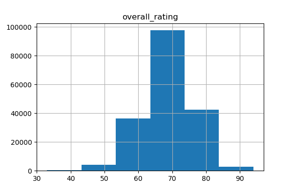
Often enough, a soccer match is determined by a single player’s moment of greatness or a single player’s costly mistake. In order to capture this, we added the number of top players and the number of bottom players as features. In order to define a top player and a bottom player, we visualized the distribution of the players’ ratings depicted in the figure below. Thus, a top player was defined with a rating greater than 80 and a bottom player was defined with a rating below 50.
A team’s current form during a season, historic home and away record, and head-to-head with the opposing team affect the players’ confidence and can indicate the stronger club. Therefore, we opted to generate multiple features that include:
- All time home (away) record - the percentage of home (away) matches that the home (away) team wins historically
- Current season home (away) record - the percentage of home (away) matches that the home (away) team has won this season
- Away record at this ground - the percentage of away matches that the away team has won at this particular ground or stadium
- Head-to-head draws - the percentage of head to head matches between the two teams that have resulted in draws
- Head-to-head home wins - the percentage of head to head matches between the two teams that have resulted in the home team winning
- Head-to-head home loss - the percentage of head to head matches between the two teams that have resulted in the home team losing
- Team offensive rating - the scraped team offensive rating data
- Team defensive rating - the scraped team defensive rating data
- Team SPI rating - the overall Soccer Power Index created by ESPN
The form guide for a team is an aggregation of its last five results. So if a team has won the last two matches, lost the two before that and drew on the one before those, its form guide will be WWLLD. A win corresponds to the letter W, a loss to the letter L, and draw to the letter D.
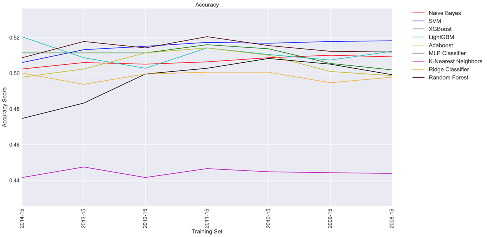
When constructing our models, we decided to train and test the models using the same approach. The dataset we have contain soccer match results for the 2008/2009 season through the 2015/2016 season. The 2015/2016 dataset had a 44.38% win rate at home, which was the baseline rate of our models. The purpose of our project is to predict the outcome of soccer games, so the accuracy of our model was tested on the final season of our data set, the 2015/2016 season. Each model was trained 7 different times and tested 7 different times. The models were first trained on the season previous 2015/2016 and tested. Next the models were trained on the previous 2, 3, 4, 5, 6, and 7 seasons and tested on the 2015/2016 season each time. The models were trained in this way so that we could compare the accuracy with the amount of data we had. This would help us understand if more data or recency of the data played a larger role in prediction accuracy.
We used a k-nearest neighbors classifier with a 5-fold cross validation and achieved an average accuracy of 44.42% from the different training sets. We tried using a k-nearest neighbors classifier because there might be some clustering within the dataset. This model did not perform well because of the weighting system it used. The weights were proportioned inverse to their distance instead of by the most important features, which caused the model to perform poorly.
The naive Bayes classifier grows a tree based on Bayes’ theorem. Using a scaler and PCA, it performs well with little computational power. This model had an average accuracy of 50.67% from the different training sets. Most of the error from this classifier came from the fact that it mostly predicted wins for every match.
We used a ridge regression classification model to analyze the multicollinearity relationship among the different features. This model achieved an average accuracy 49.81% from the different training sets. This model was helpful with feature engineering and importance. Using this model, we can create bias weightings between features of the dataset and adjust our model parameters based off of the relationships deduced. This model was one of the most simple but produced a relatively high accuracy.
Random forest is an ensemble learning method that works by building multiple decision trees during training. Unlike regular decision trees, random forests avoid overfitting the training set. With random forest, we were able to produce an average accuracy of 51.43% from the different training sets. Random forest works well for us because our final dataset has a reduced number of features, each correlating to a multiple features in the original dataset. Therefore, we reduced the number of features used while keeping the same number of samples, which is an attribute favorable for random forest classification.
We used an SVM classifier and achieved an average accuracy of 51.48%. Our model achieved the best result using the robust scaler and the first four components of the PCA transform.
Adaboost is an ensemble classifier that tries to iteratively adjust the weights of incorrectly classified examples and focuses on the more difficult cases. We used a decision tree classifier as a base estimator and tuned its hyperparameters using a 5-fold cross-validation. After training, we achieved an average accuracy of 50.50% from the different training sets. Generating the confusion matrix of the model trained on seasons 2011/12 to 2014/15, we were able to see how well the model was able to predict the different classes. The classifier predicts home wins with an accuracy of 82%, away wins with an accuracy of 47%, and draws with a low accuracy of 3%, labeling draws as home/away wins instead.
The MLP Classifier is a neural network classifier with hidden layers that map a set of inputs onto a set of appropriate outputs. After testing and tuning, the logistic sigmoid function was used as an activation function and the Broyden-Fletcher-Goldfarb-Shanno (BFGS) algorithm, an iterative quasi-Newton method for approximating the nonlinear weights, was used for weight optimization. The MLP Classifier was set to 2 hidden layers in order to avoid overfitting. After tuning, the model achieved an average accuracy of 49.60%.
XGBoost is the most common solution for gradient boosting, which is used in many cases very successfully. After tuning the model using 5-fold cross-validation, the model achieved an average accuracy of 51.01% across the different training sets.
LightGBM is a gradient boosting framework made by Microsoft. It is newer than XGBoost and has a different approach to growing trees. After tuning the model using 5-fold cross-validation, the model achieved an average accuracy of 51.08%.
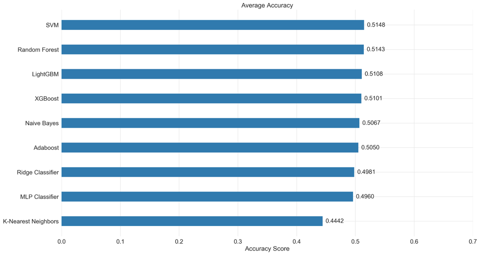
We compiled the accuracy that every model achieved across the different datasets into a table. We also made a graph that compiles the results of the different models into a form that is more digestible. The LightGBM and random forest models gave the highest accuracy of around 52% for their best results. For the random forest classifier, we reached its maximum accuracy with four training seasons. For the LightGBM model we only needed one season. Based on average performance, the SVM classifier outperformed every other model. Also based on average performance, the k-nearest neighbors classifier performed the worst.
| Training 2014-15 | Training 2013-15 | Training 2012-15 | Training 2011-15 | Training 2010-15 | Training 2009-15 | Training 2008-15 | |
|---|---|---|---|---|---|---|---|
| Naive Bayes | 50.23% | 50.59% | 50.50% | 50.63% | 50.86% | 51.00%* | 50.91% |
| SVM | 50.59% | 51.31% | 51.50% | 51.72% | 51.67% | 51.77% | 51.81%* |
| XGBoost | 51.13% | 51.13% | 51.13% | 51.59%* | 51.36% | 50.54% | 50.18% |
| LightGBM | 52.03%* | 50.86% | 50.27% | 51.41% | 51.04% | 50.73% | 51.22% |
| AdaBoost | 49.77% | 50.23% | 51.13% | 51.41%* | 51.00% | 50.09% | 49.86% |
| MLP Classifier | 47.46% | 48.32% | 49.95% | 50.27% | 50.82%* | 50.50% | 49.91% |
| K Nearest Neighbors | 44.15% | 44.74% | 44.15% | 44.65% | 44.47%* | 44.42% | 44.38% |
| Ridge Classifier | 50.00% | 49.37% | 49.95% | 50.05% | 50.05%* | 49.46% | 49.77% |
| Random Forest | 50.86% | 51.77% | 51.41% | 52.04%* | 51.54% | 51.22% | 51.18% |
*denotes highest accuracy for each model
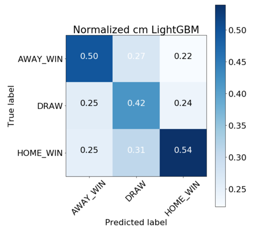
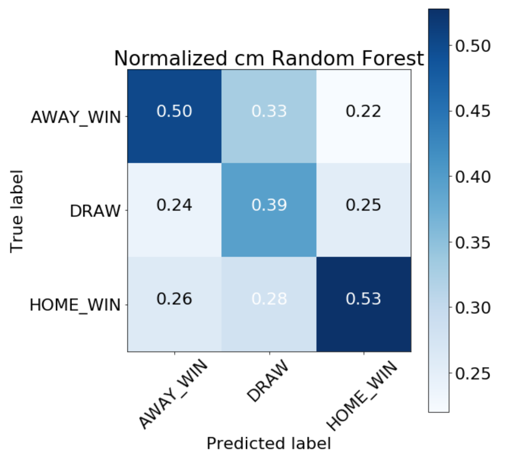
We achieved our best results with the LightGBM and random forest models. From the absolute confusion matrices below we can see that it’s difficult for both models to predict draws. Furthermore, the random forest classifier predicts a higher rate of home wins than the LightGBM model.
 |
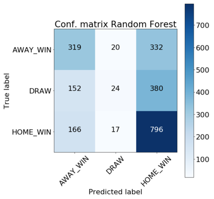 |
Taking a look at the test dataset, it is important to establish percentage guidelines for each of the three classes. We can compare the values below to our normalized confusion matrices to see how well our model performed.
| Away Win | Draw | Home Win |
|---|---|---|
| 25.20% | 30.42% | 44.38% |
 |
 |
In conclusion, it is very difficult to predict the outcome of soccer games. We were able to achieve an accuracy of 52% solely using the data from Kaggle and the features we engineered and scraped. In comparison to the prediction accuracy of the most accurate betting website, which was 53%, this model performed well. Considering the fact that soccer betting websites employ the use of professional sports analysts, and our team didn’t have any professional sports analysts, our model was exceptional.
The first step in continuing work on this project would be collecting Twitter sentiment data on teams leading up to their matches. Work has already commenced on collecting Twitter data but due to the Twitter API rate limit, there wasn’t enough time to collect all of the data. The next step for future work would be to capture model performance on a country-by-country basis. This would allow us to see the variance in data between the results of soccer games in different countries. Another possible step in future work would be to test our model accuracy as games occur. We could then ensemble this data to our existing model to improve the results of our model. A fourth step for possible future work would be to test betting earnings of our model. For a game-by-game basis, we could bet a fixed amount on the team our model predicts and record our earnings after one season. A final step in future work on this project would be to tune our models further, which would produce better results.
[1] “Global sports market revenue 2005-2017 | Statistic.” Statista, www.statista.com/statistics/370560/worldwide-sports-market-revenue/.
[2] “Top 10 List of the World's Most Popular Sports.” World's Most Popular Sports by Fans, www.topendsports.com/world/lists/popular-sport/fans.htm.
[3] Mathien, Hugo. European Soccer Database | Kaggle, 23 Oct. 2016, www.kaggle.com/hugomathien/soccer.
[4] Projects.fivethirtyeight.com. (2017). [online] Available at: https://projects.fivethirtyeight.com/global-club-soccer-rankings/ [Accessed 12 Dec. 2017].
[5] Borjigin, K. "Players FIFA 18 Dec 11, 2017 SoFIFA". n.d., https://sofifa.com. Accessed 11 December 2017.

