-
Notifications
You must be signed in to change notification settings - Fork 2
Shortest Path algorithm for Model Train
In this document, we describe the use of Dijkstra’s algorithm to find the shortest path between two stations in a model train layout.
Modern train layout can be automatically managed by software which gives the end-user a lot of fun to see all the trains moving automatically, without collisions between the various moving trains. A train layout is divided into “blocks.” Each block is a track segment between two turnouts.
In particular, we discuss the algorithm implemented by the open-source BTrain software.
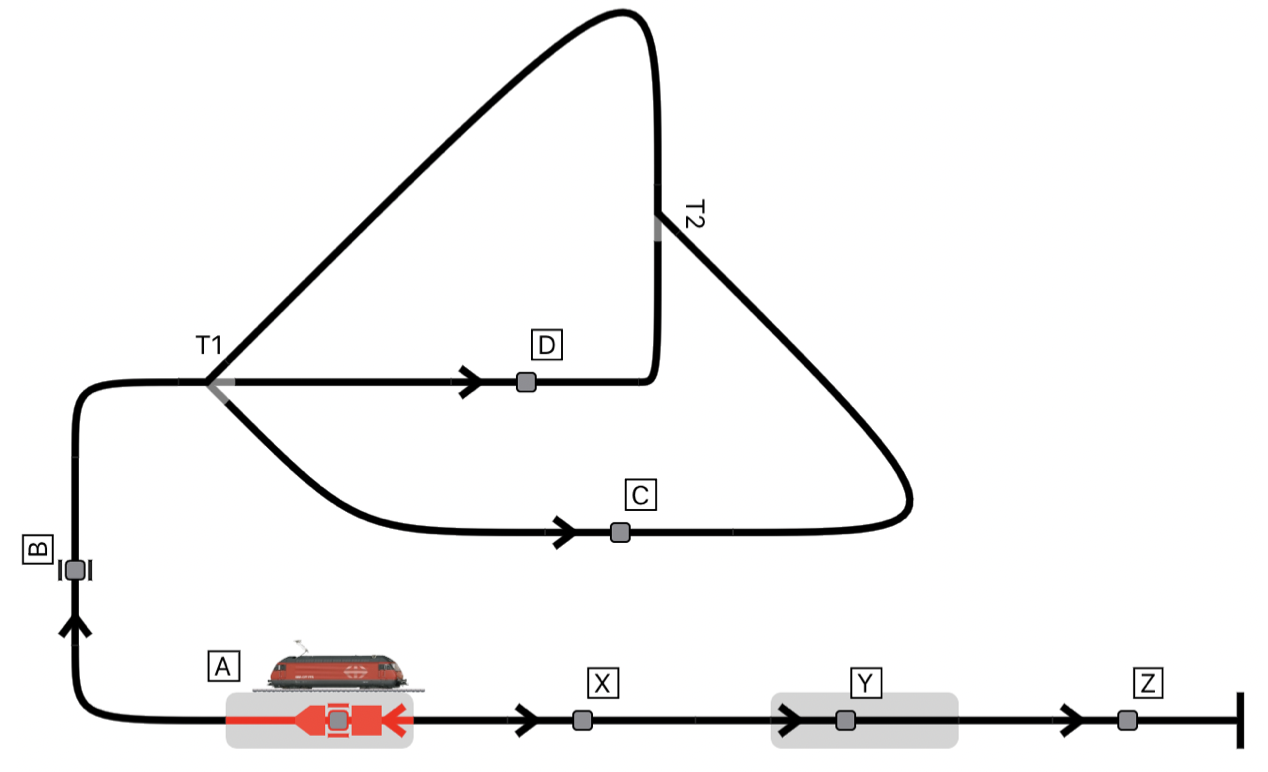
For example, the following layout has two block stations, “A” and “Y,” five “free” blocks B, C, D, X, and Z, as well as two turnouts T1 and T2. This layout is interesting because moving the train from block A to block Y is not straightforward; if the locomotive is moving in the left-side direction, it cannot go straight from A to Y via X but needs to go around the loop of T1 and T2 before coming back in the opposite direction in A to finally reach Y via X.
One feature of the software is computing the shortest path for a train to go from one station to another. Dijkstra’s shortest path algorithm works on a graph of nodes by starting at a node and recursively visiting its adjacent node, assigning “weight” to each node, representing the distance from the original node. The process repeats until all nodes are visited, choosing the node with the shortest path at each iteration.
Each node represents a block or a turnout in a model train layout.
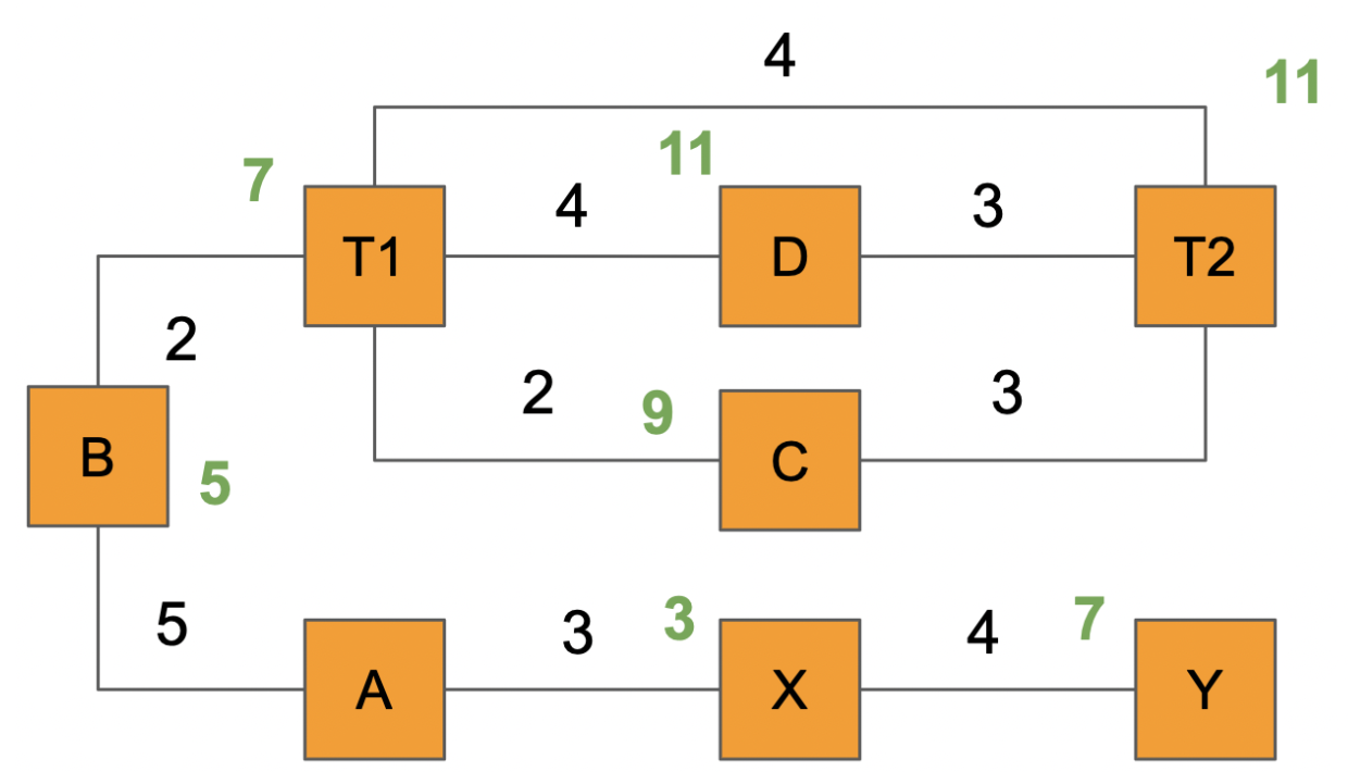
Let’s use the following graph to illustrate how Dijkstra works: let’s start with node A. All the distances between the nodes are indicated in black.
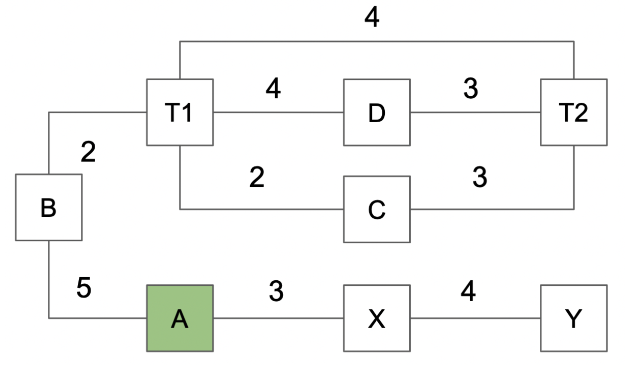
The first iteration computes the distance for the adjacent node of A, namely B and X:
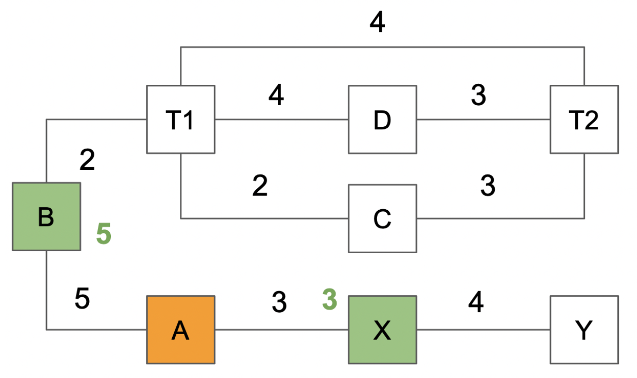
- Node B and X have their distance assigned. They are marked as “evaluated but not yet visited” in green:
- distance(X) = 3
- distance(B) = 5
- Node A is marked as “visited” in orange.
The process is repeated by taking the evaluated but not yet visited node in order of shortest distance. So X is visited first, and the distance to Y is evaluated. Then B is visited, and the distance to T1 is evaluated.
- distance(T1) = 5+2 = 7
- distance(Y) = 3+4 = 7
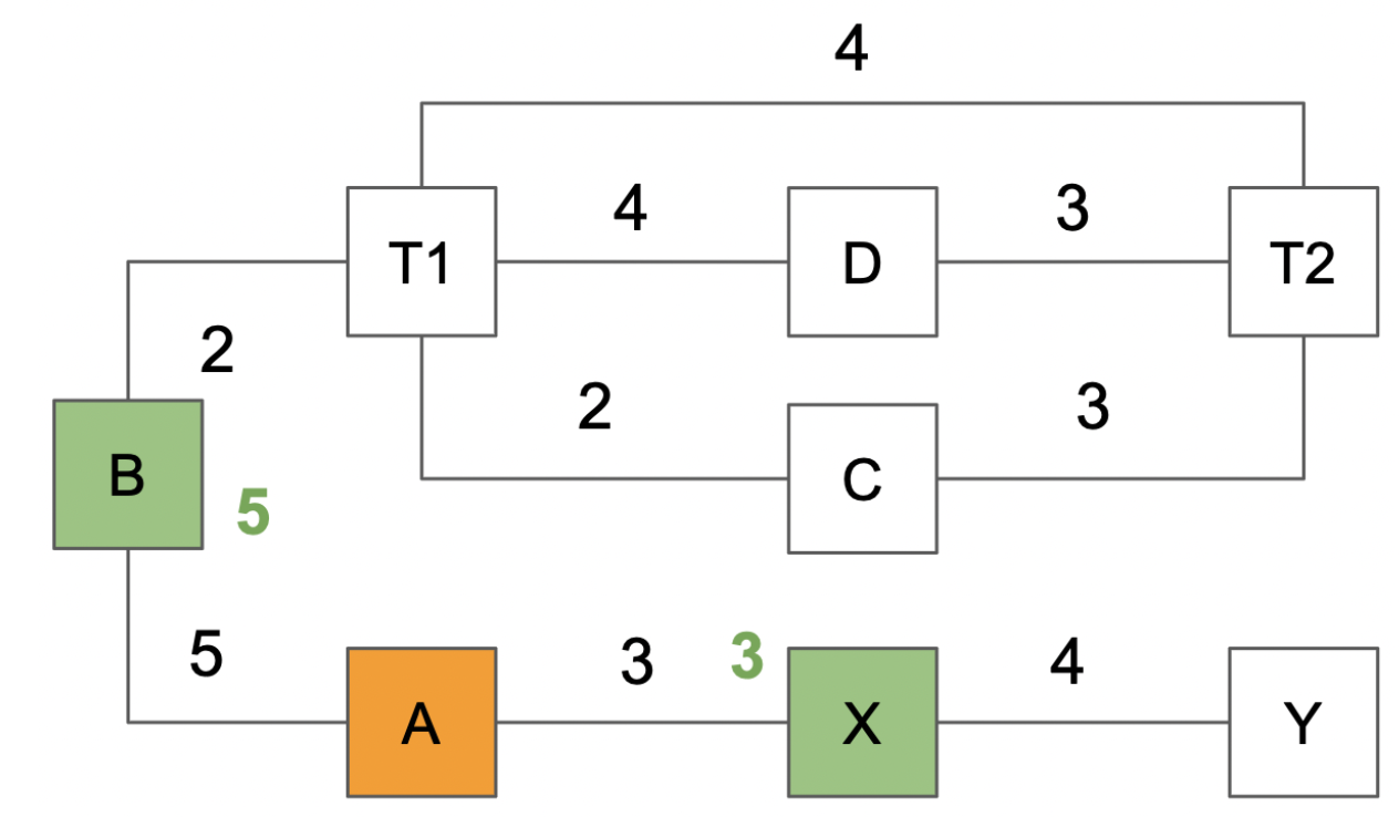
The process is repeated:
- T1 and Y are visited.
- Distances are computed for the adjacent nodes of T1 (Y does not have any adjacent node that is evaluated but not visited).
- distance(D)=7+4=11
- distance(C)=7+2=9
- distance(T2)=7+4=11
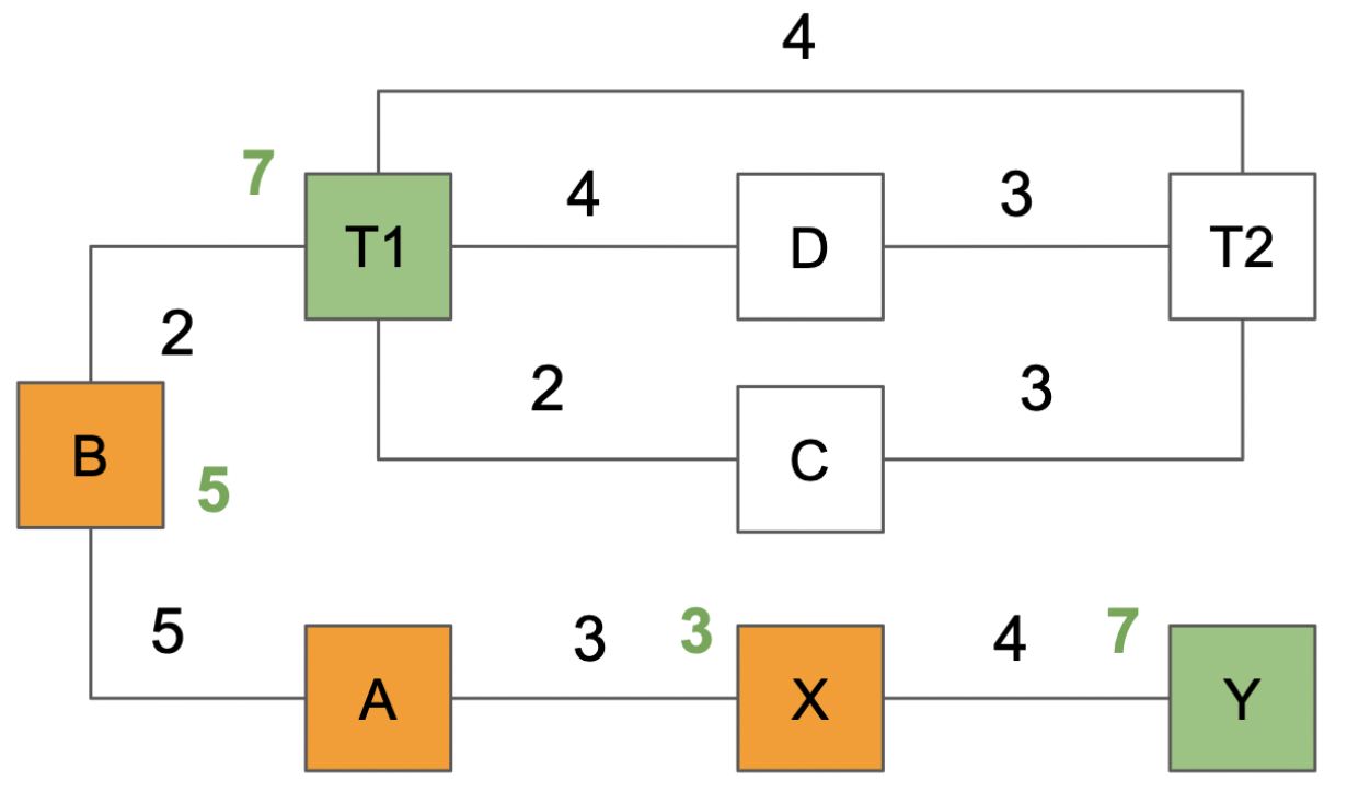
The process is repeated by picking the adjacent node that has been evaluated with the shortest distance but not yet visited.
- Node C is visited first (distance 9 is shorter than distance for D or T2)
- Distance to T2 is computed: 9+3=12 which is greater than the already evaluated distance of 11, so this new distance of 11 is discarded.
- Node D is then visited.
- Distance to T2 is computed: 11+3=14 which is greater than the existing distance of T2 of 11, so this new distance of 14 is discarded.
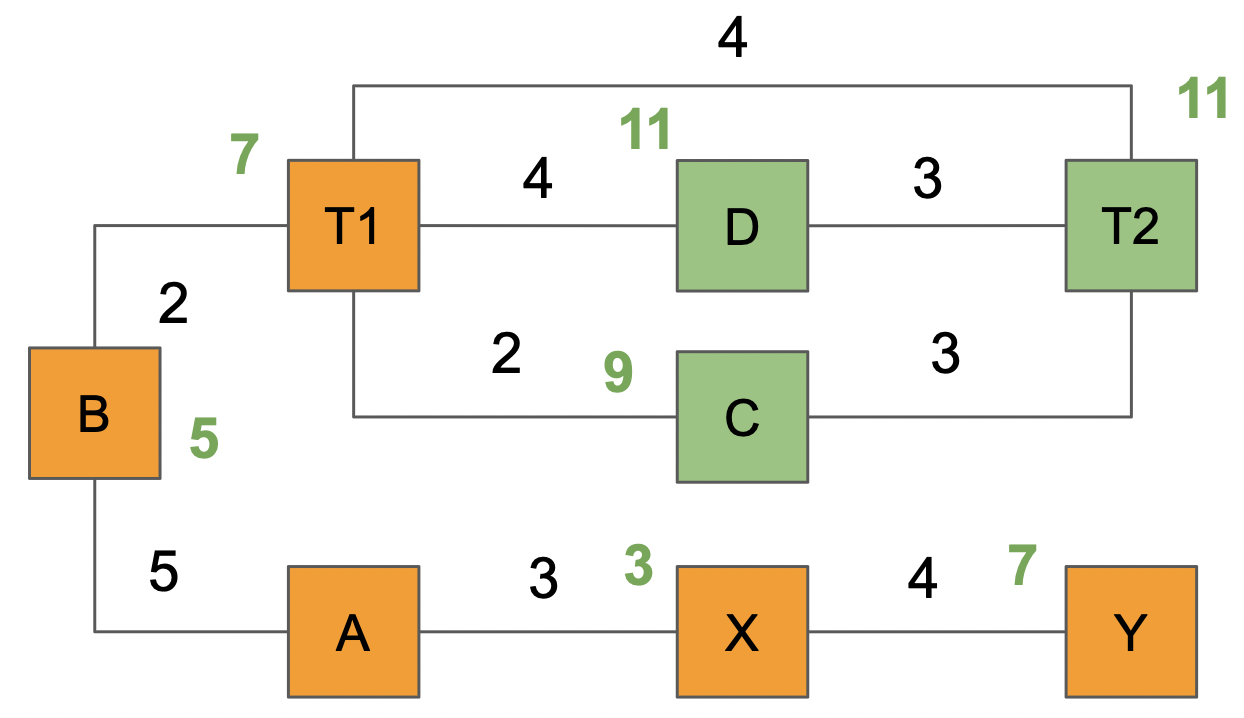
Finally, T2 is visited, and it has no more nodes to evaluate, so the process stops. At this point, the shortest paths between A and all the nodes are established. For example, going from A to T2 using the shortest path would lead to the path: A-B-T1-T2.
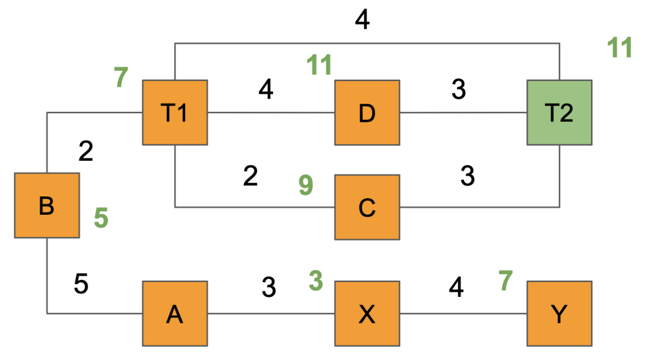
In an actual model train, it is not possible to immediately use the Dijkstra algorithm without some kind of modification. The reason is that a train cannot always move in both directions (for example, an intercity train might always move forward because of the locomotive configuration and never backward).
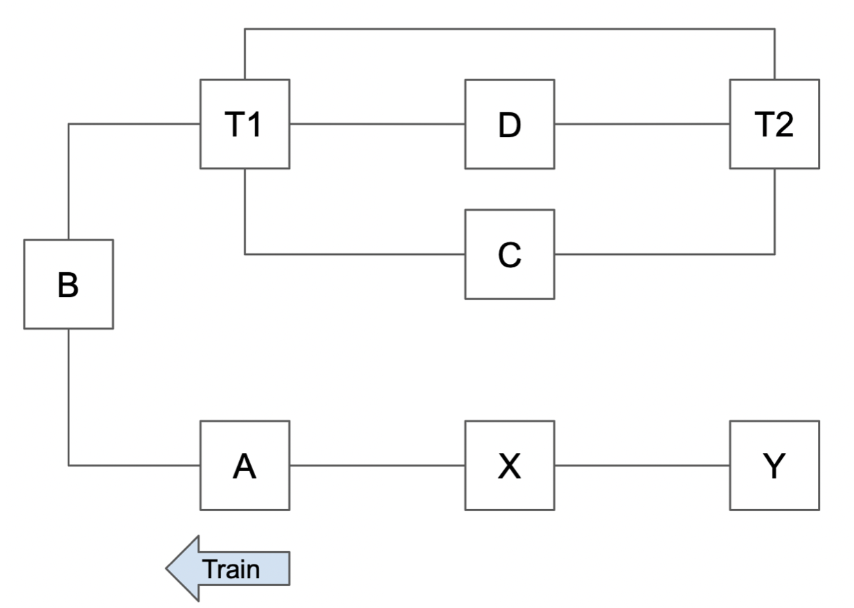
For example, a train located in node A has an arrow indicating its direction (a train moves through a block or turnout in either the “next” or “previous” direction):
Given this constraint, we immediately see that the train cannot go from A to Y via the path A-X-Y. However, this is the path that Dijkstra would return as the shortest path between A and Y.
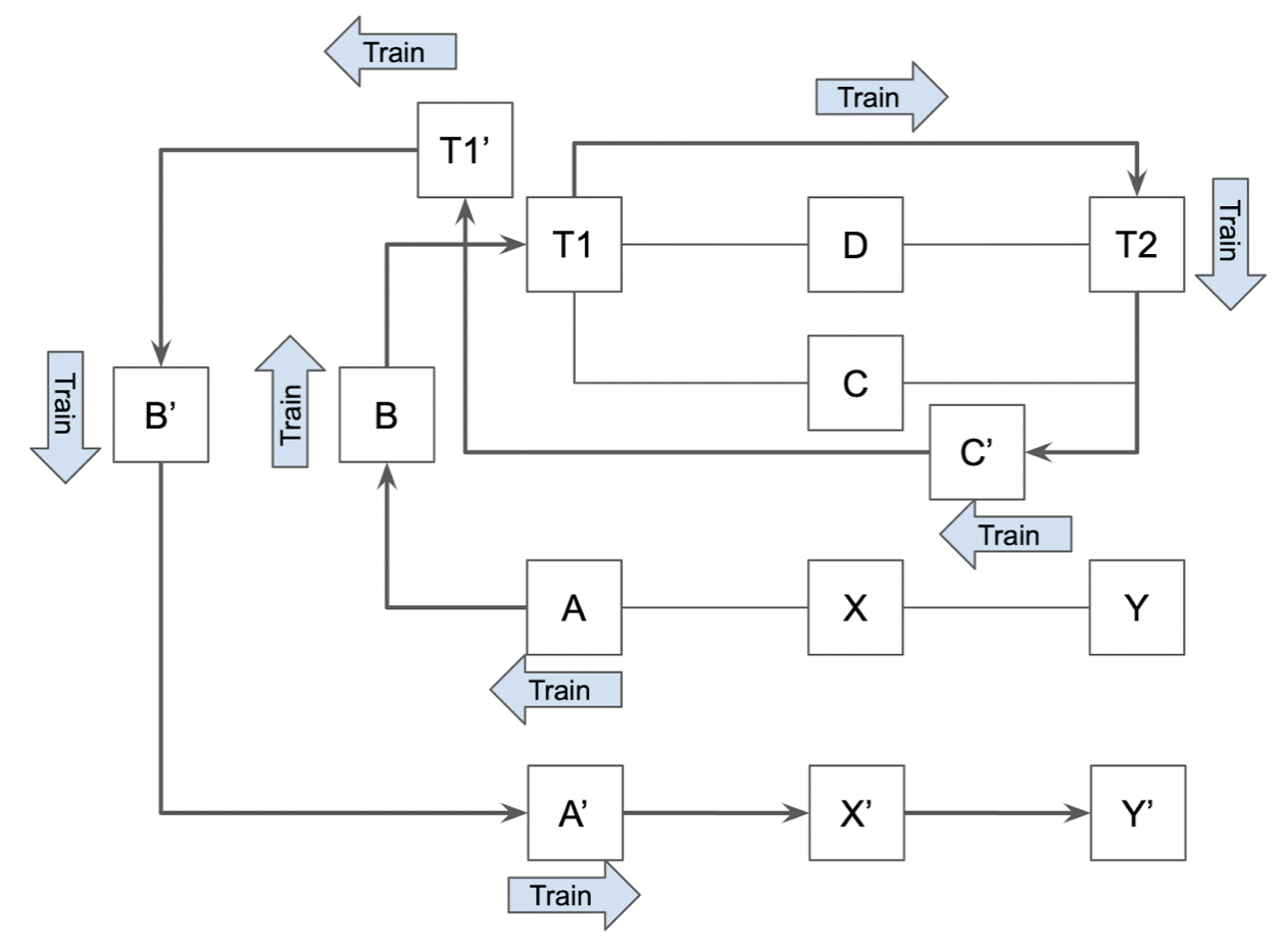
To solve this, we identify a node by its name and direction. Node (A, next) is not the same as node (A, previous). Applying this to our example, we can rerun our algorithm, which will have the effect of “unfolding” the graph:
Let’s take a look in more detail at how the algorithm proceeds:
- Starting at node (A, next).
- The only adjacent nodes reachable from (A, next) is (B, next). The train cannot move backward to reach X.
- From (B, next), the adjacent node is T1.
- From (T1), the adjacent nodes are T2, C, and D.
- Distances for nodes T2, C, and D are evaluated.
- T2 is found to have the shortest path directly from T1.
- We would stop at T2 in the regular algorithm because no more un-visited adjacent nodes can be found. However, C, D, and T1 can be revisited in this case because the train can reach out to these nodes in the opposite direction (C, previous), (D, previous), or (T1, previous). These nodes are indicated as C’, D’, and T’.
- Continuing from B’, the train can go to A’.
- From A’, this time, the train can reach X’.
- From X’, the train can reach Y’.
To move from A to Y, the train needs to take the (shortest) path A-B-T1-C-D-B’-A’-X’-Y’.
Here is a screenshot of the actual layout with the first portion of the shortest path reserved (in orange) for the train:
