The fitting program is written in python. I recommend installing the anaconda distribution of python. You will need to use python3 and will also need a few common libraries installed. The libraries you will need are:
- Numpy
- Matplotlib
- SciPy
- Pandas
These python programs are used to perform a fitting of the equations that describe peak intensities as a function of R1 relaxation, exchange rate (k) and exchange (mixing) time between two slowly exchanging conformations. In the Farrow paper below, these confirmations are labeled 'n' and 'u' (native versus unfolded). The nomenclature used for this fitting software is state 'A' and state 'B'. Four peaks appear in these experiments for each exchanging system. The intensity of these four peaks are labeled as:
- IAA: The intensity of system A that is recorded at position A
- IBB: The intensity of system B that is recorded at position B
- IAB: The intensity of system A that has moved to position B
- IBA: The intenisty of system B that has moved to position A
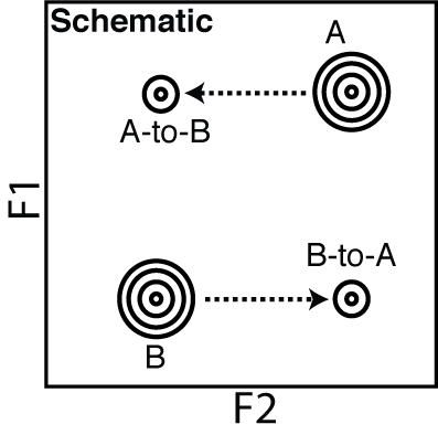
In the experiments described in the references 15N (or F1) is encoded before the exchange period, so it does not change during the mixing period. So the peak for 'A to B' is seen as a peak with the same 15N frequency as A but now has a frequency of B for 1H. This is because the system has now moved to a new 1H position and is recorded directly (F2). See schematic below.
Data files need to be in CSV format. Example files are included in the 'Example_Data' directory, e.g. H76_noise.csv. This files looks like this:
 t,IAA,IAAn,IBB,IBBn,IAB,IABn,IBA,IBAn
 0.0232,1553000,49000,816700,49000,329600,49000,233100,49000
 0.0432,1345000,49000,613200,49000,385400,49000,312600,49000
 0.0632,1208000,47000,580400,47000,458200,47000,364200,47000
 0.0832,1036000,45000,552800,45000,447300,45000,325900,45000
 0.1032,979300,44000,483200,44000,483600,44000,368200,44000
 0.1432,822400,41000,479500,41000,495600,41000,407100,41000
 0.2232,572100,37000,319100,37000,437300,37000,297200,37000
 0.3032,461800,34000,239900,34000,345300,34000,224200,34000
 0.5832,169400,25500,63770,25500,95080,25500,77400,25500
 0.8032,13060,23000,16940,23000,10,23000,10,23000
The first line gives titles to the columns - these are required. The remaining lines are exchange time (first column) and intensity data followed by noise estimate for each of the four peaks. Basically, each row is the time and then intensity data for the four peaks of an exchange system at that time point.
Nicely formated for clarity, it looks like this:
| t(sec) | IAA | IAAn | IBB | IBBn | IAB | IABn | IBA | IBAn |
|---|---|---|---|---|---|---|---|---|
| 0.0232 | 1553000 | 49000 | 816700 | 49000 | 329600 | 49000 | 233100 | 49000 |
| 0.0432 | 1345000 | 49000 | 613200 | 49000 | 385400 | 49000 | 312600 | 49000 |
| 0.0632 | 1208000 | 47000 | 580400 | 47000 | 458200 | 47000 | 364200 | 47000 |
| 0.0832 | 1036000 | 45000 | 552800 | 45000 | 447300 | 45000 | 325900 | 45000 |
| 0.1032 | 979300 | 44000 | 483200 | 44000 | 483600 | 44000 | 368200 | 44000 |
| 0.1432 | 822400 | 41000 | 479500 | 41000 | 495600 | 41000 | 407100 | 41000 |
| 0.2232 | 572100 | 37000 | 319100 | 37000 | 437300 | 37000 | 297200 | 37000 |
| 0.3032 | 461800 | 34000 | 239900 | 34000 | 345300 | 34000 | 224200 | 34000 |
| 0.5832 | 169400 | 25500 | 63770 | 25500 | 95080 | 25500 | 77400 | 25500 |
| 0.8032 | 13060 | 23000 | 16940 | 23000 | 10 | 23000 | 10 | 23000 |
You'll see that each time point has the same noise level. This could be just a single column but I havent implemented that (yet). You also don't have to have the noise estimates, but you will not be able to run Monte Carlo simulations to get an estimate of the accuracy of the fitting parameters.
N.B. - the GUI program does not work right now. Its a work in progress.
The fitting is done with a command line program called PapuaExchange.py. Execute this program with the command:
python3 PapuaExchange.py [-h] -data DATA_FILE [-plot PLOT_OUTPUT]
                         [-mc MONTE_CARLO] [-pdf PDF_PLOT]
Depending on the options, several things will happen. Firstly, in all cases the program will return the fitted parameters if they can be fitted. If the file format is wrong you will mostly get an ugly error. Check the file format. The file with the data is given with the option:
-data DATAFILE
where your CSV file name replaces DATAFILE
If you want a plot on the screen of the data and the fit use:
-plot 1 or -plot Y
If not, just leave this out or use
-plot 0
Note: If you want a pdf file saved of the fitting, you must activate a plot
To name a pdf file for saving data, use:
-pdf PDF_PLOT
where PDF_PLOT is the name of the file to save.
If you want to do a Monte Carlo Simulation to estimate how accurate you can model the parameters, use the following command
-mc MONTE_CARLO
where MONTE_CARLO is the number of simulations to run. I suggest about 50. If you dont have a noise estimate for your data or you just dont want to do a Monte Carlo simulation just leave this flag out.
You can use the Example Data in the Example_Data directory. For example, a simple fit of the data with a simple return of the parameters would be done like this:
python3 PapuaExchange.py -data Example_Data/H76.csv
or
python3 PapuaExchange.py -data Example_Data/H76_noise.csv
which will return something like:
IAA0: 2018878.1344
IBB0: 1101658.4032
R1A: 2.3819
R1B: 3.5807
k_ab: 9.6044
k_ba: 6.9073
Here, IAA0 and IBB0 are the initial (no mixing/exchange time) estimate of intensity for state A and B, respectively. R1A and R1B is an estimate of the Longtitudinal Relaxation Rate for state A and B, respectively. These numbers have units in the same units of the time numbers given in the data file (usually seconds). k_ab and k_ba are estimates of the rate of exchange from A to B and B to A, respectively. Again, the units of this time parameter is the same as the units used in the data file.
The file H76.csv, which has no noise estimates in it, works fine here because we don't do a Monte Carlo Simulation. But a file with noise esitmates works as well, so long as the first line of the CSV file is accurately labeled.
Now, lets do a full Monte Carlo Simulation with plotting and writing a PDF file. Try:
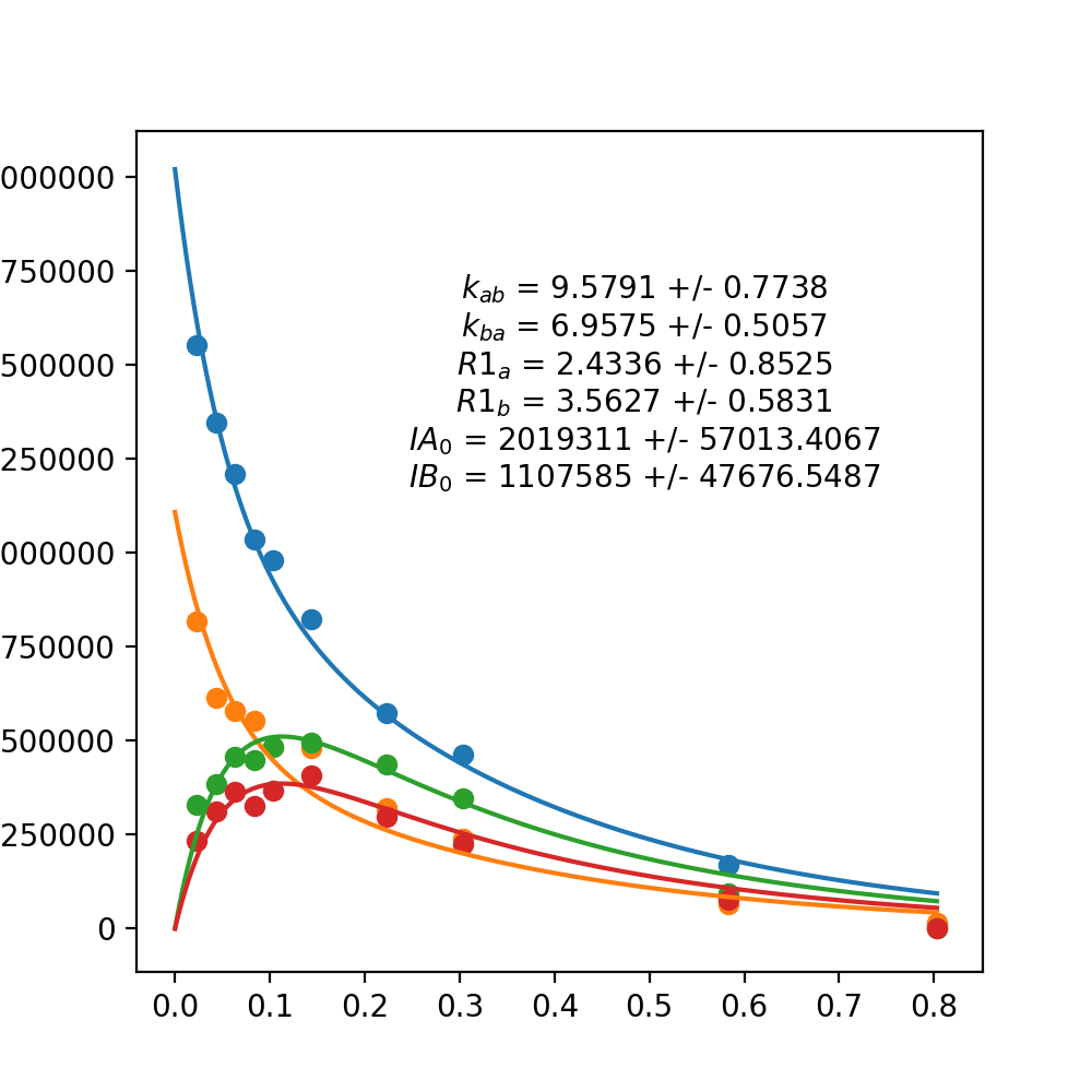
python3 PapuaExchange.py -data Example_Data/H76_noise.csv -mc 50 -plot 1 -pdf H76_Monte_Carlo
There is no need to add a .pdf to the end of a file name, it will be added anyway. This plots on the screen the data and fit and also saves a pdf file called H76_Monte_Carlo.pdf.
It should something like this:
References:
Farrow N, Zhang O, Forman-Kay J, Kay L. (1994) A heteronuclear correlation experiment for simultaneous determination of 15N longitudinal decay and chemical exchange rates of systems in slow equilibrium. J. Biomol. NMR. 4(5) 727-34.
Robson, S.A., Peterson, R., Bouchard, L.S., Villareal, V.A., Clubb, R.T. (2010) A heteronuclear zero quantum coherence Nz-exchange experiment that resolves resonance overlap and its application to measure the rates of heme binding to the IsdC protein. J. Am. Chem. Soc. 132, 9522-3.

